import sympy
q = sympy.Symbol('q')
d = sympy.Symbol('d')
L = sympy.Symbol('L')
P = sympy.Symbol('P')
h = sympy.Symbol('h')
b = sympy.Symbol('b')
E = sympy.Symbol('E')
x = sympy.Symbol('x')
subs = {}
#subs[k]=1000
subs[P]=.1
subs[L]=.1
subs[b]=.01
subs[h]=.01
subs[E]=1e7
subs[x]=.5
Approximating a cantilever with a single revolute joint
Arbitrarily placing a compliant joint halfway along its length can be used to approximate a cantilever beam.
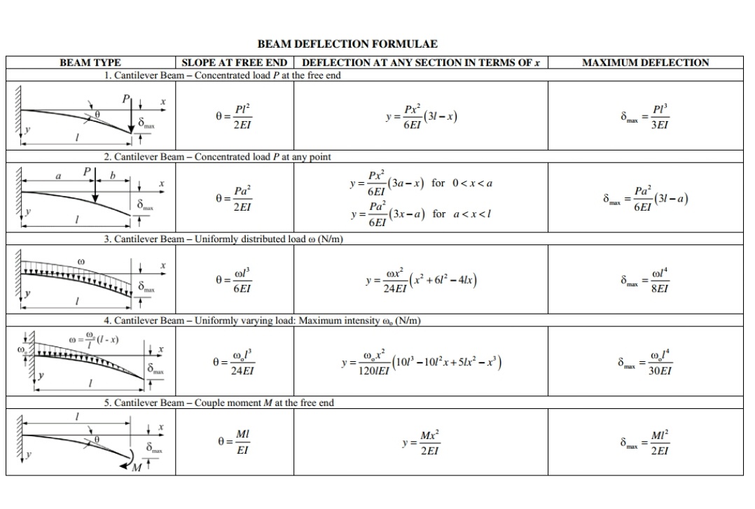
Euler-Bernoulli Equations
Point Load at the end:
$$d = \frac{PL^3}{3EI}$$
Cross-sectional moment of inertia for a rectangle
$$I = \frac{bh^3}{12}$$
Inserted: $$d = \frac{4PL^3h^3}{Eb}$$
$$E_{rectangle} = \frac{4PL^3h^3}{db}$$ $$E = \frac{PL^3}{3dI}$$
Cross sectional moment of inertia for a rectangle
I = b*h**3/12
d1 = P*L**3/3/E/I
d1.subs(subs)
$\displaystyle 0.004$
q1 = P*L**2/2/E/I
q1.subs(subs)
$\displaystyle 0.06$
2-Link Approximation
Matching Displacement
x at .5
$$d = L(1-x) \sin{\theta}$$
$$\tau=k\theta = PL(1-x)\cos\theta $$
Using a small Angle approximation, $\cos\theta = 1$
$$k\theta = PL(1-x)$$ $$\theta = \frac{PL(1-x)}{k}$$ $$d=L(1-x)\sin\left(\frac{PL(1-x)}{k}\right)$$
$$d=L(1-x)\sin\left(\frac{PL(1-x)}{k}\right)=\frac{PL^3}{3EI}$$ $$(1-x)\sin\left(\frac{PL(1-x)}{k}\right)=\frac{PL^2}{3EI}$$
$$\frac{PL(1-x)}{k}=\sin^{-1} \left(\frac{PL^2}{3EI(1-x)}\right)$$
$${k}=\frac{PL(1-x)}{\sin^{-1} \left(\frac{PL^2}{3EI(1-x)}\right)}$$
k1 = P*L*(1-x)/(sympy.asin(P*L**2/(3*E*I*(1-x))))
k1.subs(subs)
$\displaystyle 0.0624332120451467$
The displacement matches
d2 = L*(1-x)*sympy.sin(P*L*(1-x)/k1)
d2.subs(subs)
$\displaystyle 0.004$
But the orientation does not
q2 = P*L*(1-x)/k1
q2.subs(subs)
$\displaystyle 0.080085580033659$
Matching Theta
From Cantilever beam equations:
$$\theta = \frac{PL^2}{2EI}$$
From approximation above, again assuming small angles:
$$\theta = \frac{PL(1-x)}{k}$$
$$\theta = \frac{PL^2}{2EI}= \frac{PL(1-x)}{k}$$ $$\frac{L}{2EI}= \frac{1-x}{k}$$ $$k=\frac{2EI(1-x)}{L}$$
Using the value solved for to equate orientation:
k2 = 2*E*I*(1-x)/(L)
Now orientation matches
q3 = P*L*(1-x)/k2
q3.subs(subs)
$\displaystyle 0.06$
But displacement does not
d3 = L*(1-x)*sympy.sin(P*L*(1-x)/k2)
d1.subs(subs)
$\displaystyle 0.004$
d3.subs(subs)
$\displaystyle 0.00299820032397223$
Matching Both
Now asking the question, what location x permits you to accurately model the deflection and angle of a cantilever beam with a single joint?
del subs[x]
Create an error vector
error = []
error.append(d1-d2)
error.append(q1-q2)
error= sympy.Matrix(error)
error = error.subs(subs)
error
$\displaystyle \left[\begin{matrix}0\0.06 - \operatorname{asin}{\left(\frac{0.04}{1 - x} \right)}\end{matrix}\right]$
import optimization toolkit
import scipy.optimize
Turn “error” into a function that can be run using the sympy.lambdify function
f = sympy.lambdify((x),error)
Scipy.optimize.minimize needs args supplied as a list, so define a new wrapper function that formats inputs correctly
def f2(args):
    a = f(*args)
    b = (a**2).sum()
    return b
sol = scipy.optimize.minimize(f2,[.25])
sol
      fun: 2.0974856866229214e-09
 hess_inv: array([[65.11062045]])
      jac: array([-8.23593665e-06])
  message: 'Optimization terminated successfully.'
     nfev: 14
      nit: 4
     njev: 7
   status: 0
  success: True
        x: array([0.33242421])
Now add x back to the list of substitutions
subs[x]=sol.x[0]
So a virtual joint at x=1/3 correctly approximates displacement and orientation.
d2.subs(subs)
$\displaystyle 0.004$
q2.subs(subs)
$\displaystyle 0.0599542016846748$