The relationship between the bending moment and the radius of curvature($\rho$) for a beam of Young’s modulus $E$ and cross-sectional moment of inertia(second moment of area) $I$ is given by
$$ M=-\frac{EI}{\rho} $$
Now let’s say $\omega(x)$ describes the deflection of a beam in the z direction as a function of its length, $x$. When deflections are small – assumed in the Euler-Bernoulli model, then the second derivative can serve as an approximate the radius of curvature (using the small angle approximation $\sin{\theta}=\theta$), making
$$\frac{1}{\rho} = \frac{\delta^2\omega}{\delta x^2}$$
and
$$M = -EI\frac{\delta^2 \omega(x)}{\delta x^2}$$
$$\frac{\delta^2}{\delta x^2}\left(EI\frac{\delta^2 \omega(x)}{\delta x^2}\right) = p(x)$$
where $p$ is a distributed load, $E$ is Young’s Modulus, and $I$ is the
$$\frac{\delta^2 \omega}{\delta x^2} =\frac{M}{EI}$$
where $M$ is the moment,
%matplotlib inline
# -*- coding: utf-8 -*-
"""
copyright 2016-2017 Dan Aukes
"""
import matplotlib.pyplot as plt
import sympy
import numpy
from sympy import pi
b,h,theta,P,L,E,I,x,w,M,q,p,A,B,C,D,p0,M0=sympy.symbols('b,h,theta,P,L,E,I,x,w,M,q,p,A,B,C,D,p0,M0')
def plot_x(w,subs1=None):
    subs1 = subs1 or {}
    w = w.subs(subs1)
    unit = dict([(item,1) for item in w.atoms(sympy.Symbol) if item!=x])
    unit.update(subs1)
    w_num = w.subs(unit)
    f_w = sympy.lambdify(x,w_num)

    xn = numpy.r_[0:unit[L]:100j]
    yn = f_w(xn)

    plt.plot(xn,yn)
    plt.axis('equal')
First we need to compute $M(x)$, the moment on the beam as a function of the loading.
M_dd = p
M_d = sympy.integrate(M_dd,(x,0,x)) + A
M_d
$\displaystyle A + p x$
M = sympy.integrate(M_d,(x,0,x)) + B
M
$\displaystyle A x + B + \frac{p x^{2}}{2}$
w_d = sympy.integrate(M/E/I,(x,0,x)) + C
w_d
$\displaystyle \frac{A x^{2}}{2 E I} + \frac{B x}{E I} + C + \frac{p x^{3}}{6 E I}$
w = sympy.integrate(w_d,(x,0,x)) + D
w
$\displaystyle \frac{A x^{3}}{6 E I} + \frac{B x^{2}}{2 E I} + C x + D + \frac{p x^{4}}{24 E I}$
For a point load $P$ exerted on a beam at length ($x=l$), the moment can be expressed as:
$$M(x) = P(l-x)$$
eq1 = M_d.subs({x:L}) - P
eq2 = M.subs({x:L}) - 0
eq3 = w_d.subs({x:0}) - 0
eq4 = w.subs({x:0}) - 0
eq5 = M_dd - 0
sol =sympy.solve([eq1,eq2,eq3,eq4,eq5],(A,B,C,D,p))
sol
{A: P, B: -L*P, C: 0, D: 0, p: 0}
w2 = w.subs(sol)
w2.simplify()
$\displaystyle \frac{P x^{2} \left(- 3 L + x\right)}{6 E I}$
w_d2 = w_d.subs(sol)
w_d2.simplify()
$\displaystyle \frac{P x \left(- 2 L + x\right)}{2 E I}$
M2=M.subs(sol)
M2.simplify()
$\displaystyle P \left(- L + x\right)$
w_max = w2.subs({x:L})
w_max.simplify()
$\displaystyle - \frac{L^{3} P}{3 E I}$
Now we can turn this process into a function
def calc_beam_equations(pp,E,I,eq):
    M_dd = pp
    M_d = sympy.integrate(M_dd,(x,0,x)) + A
    M = sympy.integrate(M_d,(x,0,x)) + B
    w_d = sympy.integrate(M/E/I,(x,0,x)) + C
    w = sympy.integrate(w_d,(x,0,x)) + D

    eq1 = M_d.subs(eq[0][0]) - eq[0][1]
    eq2 = M.subs(eq[1][0]) - eq[1][1]
    eq3 = w_d.subs(eq[2][0]) - eq[2][1]
    eq4 = w.subs(eq[3][0]) - eq[3][1]
    eq = [eq1,eq2,eq3,eq4]

    sol =sympy.solve(eq,(A,B,C,D))

    w2 = w.subs(sol)
    w2 = w2.simplify()

    w_d2 = w_d.subs(sol)
    w_d2 = w_d2.simplify()

    M2=M.subs(sol)
    M2 = M2.simplify()

    return w2,w_d2,M2
Repeating the point load
eq1 = {x:L},P
eq2 = {x:L},0
eq3 = {x:0},0
eq4 = {x:0},0
eq = [eq1,eq2,eq3,eq4]
w,w_d,M = calc_beam_equations(0,E,I,eq)
plot_x(w)
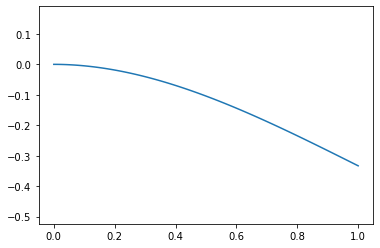
For a distibuted load $p(x)$,
eq1 = {x:L},0
eq2 = {x:L},0
eq3 = {x:0},0
eq4 = {x:0},0
eq = [eq1,eq2,eq3,eq4]
w,w_d,M = calc_beam_equations(-p,E,I,eq)
plot_x(w)
w
$\displaystyle \frac{p x^{2} \left(- 6 L^{2} + 4 L x - x^{2}\right)}{24 E I}$
w_d
$\displaystyle \frac{p x \left(- 3 L^{2} + 3 L x - x^{2}\right)}{6 E I}$
M
$\displaystyle \frac{p \left(- L^{2} + 2 L x - x^{2}\right)}{2}$
w_max = w.subs({x:L})
w_max.simplify()
$\displaystyle - \frac{L^{4} p}{8 E I}$
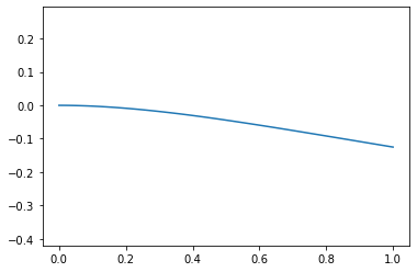
For a distributed load where $p = p_0\frac{L-x}{L}$, the boundary conditions stay the same but the function is different
w,w_d,M = calc_beam_equations(-(p0/L*(L-x)),E,I,eq)
plot_x(w)
w
$\displaystyle \frac{p_{0} x^{2} \left(5 L \left(- 2 L^{2} + 2 L x - x^{2}\right) + x^{3}\right)}{120 E I L}$
w_d
$\displaystyle \frac{p_{0} x \left(2 L \left(- 2 L^{2} + 3 L x - 2 x^{2}\right) + x^{3}\right)}{24 E I L}$
M
$\displaystyle \frac{p_{0} \left(L \left(- L^{2} + 3 L x - 3 x^{2}\right) + x^{3}\right)}{6 L}$
w_max = w.subs({x:L})
w_max.simplify()
$\displaystyle - \frac{L^{4} p_{0}}{30 E I}$
eq1 = {x:L},P
eq2 = {x:L},0
eq3 = {x:0},0
eq4 = {x:0},0
eq = [eq1,eq2,eq3,eq4]
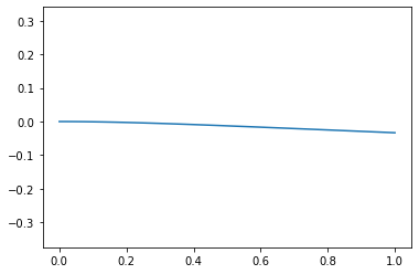
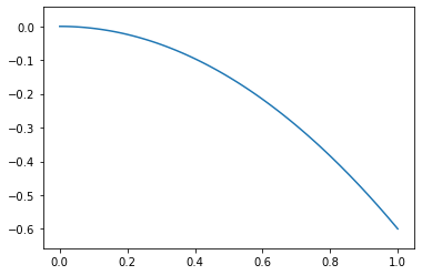
Now what about a cross sectional area that changes as a function of x? As we know, the cross sectional moment of inertia $I$ for a rectangular beam of width $b$ and thickness $h$ is $$I=\frac{bh^3}{12}$$. If we make b a function of x, for example $b(x)=L-x$, what happens to the curvature?
b2=(L-x)
I2 = b2*h**3/12
w,w_d,M = calc_beam_equations(0,E,I2,eq)
plot_x(w,{P:.1,L:1})
w
$\displaystyle - \frac{6 P x^{2}}{E h^{3}}$
w_d
$\displaystyle - \frac{12 P x}{E h^{3}}$
M
$\displaystyle P \left(- L + x\right)$
As you can see it grows linearly as a function of x. Therefore, a cross section that decreases linearly is good at equalizing the radius of curvature (and the stresses) in a beam
eq1 = {x:L},P
eq2 = {x:L},0
eq3 = {x:0},0
eq4 = {x:0},0
eq = [eq1,eq2,eq3,eq4]
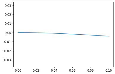
I2 = b*h**3/12
w,w_d,M = calc_beam_equations(0,E,I2,eq)
subs1 = {b:.01,h:.01,E:1e7,L:.1,P:.1}
w = w.subs(subs1)
w
$\displaystyle 2.0 x^{2} \left(x - 0.3\right)$
w_max = w.subs({x:.1})
w_max
$\displaystyle -0.004$
plot_x(w,subs1)