Kinematics with Python
Individual Assignment
Assignment Overview
The purpose of this assignment is to get you comfortable using the computational capabilities of Python and Sympy to start estimating the performance of your design.
Rubric
| Description | Points |
|---|---|
| 1. | 10 |
| 2. | 10 |
| 3. | 10 |
| 4. | 10 |
| 5. | 10 |
| 6. | 10 |
| 7. | 10 |
| 8. | 10 |
| 9. | 10 |
| 10. | 10 |
| 11. | 10 |
| 12. | 10 |
| 13. | 10 |
| 14. | 10 |
| 15. | 10 |
| Discussion | 50 |
| Total | 200 |
Resources
Instructions
Create a new jupyter/colab notebook. In the first cell, paste in this version of the code you worked on in class:
%matplotlib inline

#import required packages
import pynamics
from pynamics.frame import Frame
from pynamics.system import System
import numpy
import sympy
import matplotlib.pyplot as plt
plt.ion()
from math import pi

#-----------------------

# Create a Pynamics System
system = System()
pynamics.set_system(__name__,system)

#-----------------------
# Import Variable Types
from pynamics.variable_types import Differentiable,Constant

# Create Constants
lA = Constant(1,'lA',system)
lB = Constant(1,'lB',system)
print(system.constant_values)

# Create Differentiable State Variables
qA,qA_d,qA_dd = Differentiable('qA',system)
qB,qB_d,qB_dd = Differentiable('qB',system)

#-----------------------
# Define A Configuration

state1 = {}
state1[qA]=15*pi/180
state1[qB]=15*pi/180

#-----------------------
#Define Frames

N = Frame('N',system)
A = Frame('A',system)
B = Frame('B',system)

# Define "N" as the Newtonian Frame
system.set_newtonian(N)

# Rotate A from N about their shared z axis by amount "qA"
A.rotate_fixed_axis(N,[0,0,1],qA,system)

# Rotate B from A about their shared z axis by amount "qB"
B.rotate_fixed_axis(A,[0,0,1],qB,system)

#-----------------------
Make a new cell. create a new dictionary,
state2, in the same waystate1is defined.- Select your own values for the positions of $q_A$ and $q_B$ for
state2.
- Select your own values for the positions of $q_A$ and $q_B$ for
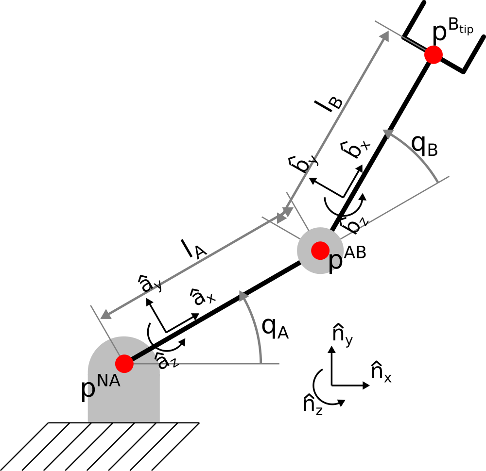
Create a new vector to describe the origin, $\vec{p}^{NA}$, which is equal to $\vec{p}^{NA} = 0 \hat{n}_x+0 \hat{n}_y+0 \hat{n}_z$.
it is necessary to describe it in this way so you are creating a vector $\vec{0}$ rather than a scalar $0$
Create a new vector to describe the point between the A link and the B link, $\vec{p}^{AB}$, which is equal to $\vec{p}^{AB} = \vec{p}^{NA}+l_A\hat{a}_x$
Create a new vector for the end effector, $\vec{p}^{B_{tip}}$, which is equal to $\vec{p}^{B_{tip}} = \vec{p}^{AB}+l_B\hat{b}_x$
Create a python
list()namedpointsof $\vec{p}^{NA}$,$\vec{p}^{AB}$,$\vec{p}^{B_{tip}}$Using the
forkeyword in Python, iterate throughpointsand dot each element with $\hat{n}_x$, saving the new list aspxHint: look up Python “list comprehensions” to do this efficiently.
- Using the
.subs()method, substitute out all symbolic variables using thesystem.constant_valuesandstate1dictionaries, saving the list as px1. This list should contain values of literal numbers with no symbols. - Using the
.subs()method, substitute out all symbolic variables using thesystem.constant_valuesandstate2dictionaries, saving the list as px2. This list should contain values of literal numbers with no symbols.
- Using the
Repeat step 6.1 with $\hat{n}_y$, saving the lists as
py,py1,andpy2
In the same figure, plot
px1vspy1in blue andpx2vspy2in red, using theplt.plot()function- Set the axes to equal proportion using the method from your first Python assignment.
use the
.time_derivative()method of $\vec{p}^{B_{tip}}$ to take the time derivative of $\vec{p}^{B_{tip}}$ to obtain $\vec{v}^{B_{tip}}$, where:$$\vec{v}^{B_{tip}}=\dot{\vec{p}}^{B_{tip}} = \frac{d^{N}(\vec{p}^{B_{tip}})}{dt}$$
with reference to the Newtonian frame, $N$. In the above expression, the $d^N$ denotes the derivative with reference to the $N$ frame.
Note: the
.time_derivative()method takes two optional keyword variables: first, the frame of reference you are taking the derivative in (it default’s to the declared Newtonian frame), and second, the current pynamics system. You may keep these optional terms blank in this case.Obtain the scalar components of $\vec{v}^{B_{tip}}$ in the $\hat{n}_x$ and $\hat{n}_y$ directions, and save as $v^{B{tip}}_x,v^{B{tip}}_y.
Use the
sympy.Matrix()function to create a 2x1 matrix $\textbf{v}$, where $$\textbf{v}=\left[\begin{array}{c} v^{B{tip}}_x \\ v^{B{tip}}_y \end{array}\right]$$Use the
sympy.Matrix()function to create a 2x1 matrix $\dot{\textbf{q}}$ (orq_din python), where$$\dot{\textbf{q}}=\left[\begin{array}{c} \dot{q}_A \\ \dot{q}_B \end{array}\right]$$
Use the
.jacobian()method of $\textbf{v}$ to compute its Jacobian $\textbf{J}$ with respect to $\dot{\textbf{q}}$. (This should result in a 2x2 matrix).Using the
.subs()method of $\textbf{J}$, identify the numerical value of new variables $\textbf{J}_1$ and $\textbf{J}_2$, by substitutingsystem.constant_valuesand then eitherstate1orstate2. This will result in two new 2x2 arrays with number literals (rather than a symbolic expression).Using $\textbf{J}_1$, $\textbf{J}_2$, and $\dot{\textbf{q}}=\left[\begin{array}{c}3.3 \\ 2.4\end{array}\right]$, identify $\textbf{v}_1$ and $\textbf{v}_2$
Now, assume that a force $\vec{f}$, formulated as a
sympy.Matrix(), where$$\textbf{f}=\left[\begin{array}{c}1.4 \\ 2.6\end{array}\right]$$ is applied to the end-effector. Compute the torques at the robot’s joints at both
state1andstate2.
Discussion
- Why are $\textbf{J}_1$ and $\textbf{J}_2$ different?
- Why is possible to determine the torques on each joint of the mechanism due to $\vec{f}$, but not to arbitrarily apply any 3D force vector on the world given the kinematics described above in your code?
- What about the structure or content of $\textbf{J}$ tells you this?
- What is the meaning of a row of zeros in $\textbf{J}$?
- What is the meaning of a column of zeros in $\textbf{J}$?
Final Submission
Please include a Jupyter notebook and pdf with the following:
- Detailed description of the completed steps above (included as blocks alongside chunks of related code)
- Code used in solving the problem (inline in the report in code blocks), along with descriptions detailing your approach.
- Detailed answers to the discussion questions, included at the bottom.
Please follow the “Submission Best Practices” document posted on Canvas. This assignment should be submitted to canvas as a .pdf document as well as a jupyter notebook (.ipynb). If submitted as a notebook, make sure it is fully compiled. This can be done by opening the file in the jupyter browser and in the top jupyter menu selecting “Kernel” –> “Restart and Run All”.